
2. Spatial relationships
2.1 Shapely geometries and spatial relationships
2.1.1 Creating a Point geometry
The Eiffel Tower is an iron lattice tower built in the 19th century, and is probably the most iconic view of Paris.
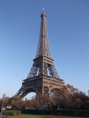
(By couscouschocolat [CC BY 2.0], via Wikimedia Commons)
The location of the Eiffel Tower is: x of 255422.6 and y of 6250868.9.
# Import the Point geometry
from shapely.geometry import Point

# Construct a point object for the Eiffel Tower
eiffel_tower = Point(255422.6, 6250868.9)

# Print the result
print(eiffel_tower)
# POINT (255422.6 6250868.9)
2.1.2 Shapely’s spatial methods
Now we have a shapely Point object for the Eiffel Tower, we can use the different methods available on such a geometry object to perform spatial operations, such as calculating a distance or checking a spatial relationship.
We repeated the construction of eiffel_tower, and also provide the code that extracts one of the neighbourhoods (the Montparnasse district), as well as one of the restaurants located within Paris.
# Construct a point object for the Eiffel Tower
eiffel_tower = Point(255422.6, 6250868.9)

# Accessing the Montparnasse geometry (Polygon) and restaurant
district_montparnasse = districts.loc[52, 'geometry']
resto = restaurants.loc[956, 'geometry']

# Is the Eiffel Tower located within the Montparnasse district?
print(eiffel_tower.within(district_montparnasse))
# False

# Does the Montparnasse district contains the restaurant?
print(district_montparnasse.contains(resto))
# True

# The distance between the Eiffel Tower and the restaurant?
print(eiffel_tower.distance(resto))
# 4431.459825587039
Note that the contains() and within() methods are the opposite of each other: if geom1.contains(geom2) is True, then also geom2.within(geom1) will be True.
2.2 Spatial relationships with GeoPandas
2.2.1 In which district in the Eiffel Tower located?
Let’s return to the Eiffel Tower example. In previous exercises, we constructed a Point geometry for its location, and we checked that it was not located in the Montparnasse district. Let’s now determine in which of the districts of Paris it is located.
The districts GeoDataFrame has been loaded, and the Shapely and GeoPandas libraries are imported.
# Construct a point object for the Eiffel Tower
eiffel_tower = Point(255422.6, 6250868.9)

# Create a boolean Series
mask = districts.contains(eiffel_tower)

# Print the boolean Series
print(mask.head())

# Filter the districts with the boolean mask
print(districts[mask])
0    False
1    False
2    False
3    False
4    False
dtype: bool

    id district_name  population                                           geometry
27  28  Gros-Caillou       25156  POLYGON ((257097.2898896902 6250116.967139574,...
2.2.2 How far is the closest restaurant?
Now, we might be interested in the restaurants nearby the Eiffel Tower. To explore them, let’s visualize the Eiffel Tower itself as well as the restaurants within 1km.
To do this, we can calculate the distance to the Eiffel Tower for each of the restaurants. Based on this result, we can then create a mask that takes True if the restaurant is within 1km, and False otherwise, and use it to filter the restaurants GeoDataFrame. Finally, we make a visualization of this subset.
The restaurants GeoDataFrame has been loaded, and the eiffel_tower object created. Further, matplotlib, GeoPandas and contextily have been imported.
# The distance from each restaurant to the Eiffel Tower
dist_eiffel = restaurants.distance(eiffel_tower)

# The distance to the closest restaurant
print(dist_eiffel.min())
# 460.6976028277898

# Filter the restaurants for closer than 1 km
restaurants_eiffel = restaurants[dist_eiffel<1000]

# Make a plot of the close-by restaurants
ax = restaurants_eiffel.plot()
geopandas.GeoSeries([eiffel_tower]).plot(ax=ax, color='red')
contextily.add_basemap(ax)
ax.set_axis_off()
plt.show()

2.3 The spatial join operation

2.3.1 Paris: spatial join of districts and bike stations
Let’s return to the Paris data on districts and bike stations. We will now use the spatial join operation to identify the district in which each station is located.
The districts and bike sharing stations datasets are already pre-loaded for you as the districts and stations GeoDataFrames, and GeoPandas has been imported as geopandas
# Join the districts and stations datasets
joined = geopandas.sjoin(stations, districts, op='within')

# Inspect the first five rows of the result
print(joined.head())
                                       name  bike_stands  available_bikes  \
0                    14002 - RASPAIL QUINET           44                4
143  14112 - FAUBOURG SAINT JACQUES CASSINI           16                0
293               14033 - DAGUERRE GASSENDI           38                1
346     14006 - SAINT JACQUES TOMBE ISSOIRE           22                0
429       14111 - DENFERT-ROCHEREAU CASSINI           24                8

                                        geometry  index_right  id district_name
0     POINT (450804.448740735 5409797.268203795)           52  53  Montparnasse
143   POINT (451419.446715647 5409421.528587255)           52  53  Montparnasse
293  POINT (450708.2275807534 5409406.941172979)           52  53  Montparnasse
346  POINT (451340.0264470892 5409124.574548723)           52  53  Montparnasse
429  POINT (451274.5111513372 5409609.730783217)           52  53  Montparnasse
2.3.2 Map of tree density by district (1)
Using a dataset of all trees in public spaces in Paris, the goal is to make a map of the tree density by district. For this, we first need to find out how many trees each district contains, which we will do in this exercise. In the following exercise, we will then use this result to calculate the density and create a map.
To obtain the tree count by district, we first need to know in which district each tree is located, which we can do with a spatial join. Then, using the result of the spatial join, we will calculate the number of trees located in each district using the pandas ‘group-by’ functionality.
GeoPandas has been imported as geopandas.
# trees
      species location_type                                     geometry
0  Marronnier    Alignement  POINT (455834.1224756146 5410780.605718749)
1  Marronnier    Alignement  POINT (446546.2841757428 5412574.696813397)
2  Marronnier    Alignement    POINT (449768.283096671 5409876.55691999)
3  Marronnier    Alignement   POINT (451779.7079508423 5409292.07146508)
4     Sophora    Alignement  POINT (447041.3613609616 5409756.711514045)
# Read the trees and districts data
trees = geopandas.read_file("paris_trees.gpkg")
districts = geopandas.read_file("paris_districts_utm.geojson")

# Spatial join of the trees and districts datasets
joined = geopandas.sjoin(trees, districts, op='within')

# Calculate the number of trees in each district
trees_by_district = joined.groupby('district_name').size()

# Convert the series to a DataFrame and specify column name
trees_by_district = trees_by_district.to_frame(name='n_trees')

# Inspect the result
print(trees_by_district.head())
                 n_trees
district_name
Amérique             183
Archives               8
Arsenal               60
Arts-et-Metiers       20
Auteuil              392
2.3.3 Map of tree density by district (2)
Now we have obtained the number of trees by district, we can make the map of the districts colored by the tree density.
For this, we first need to merge the number of trees in each district we calculated in the previous step (trees_by_district) back to the districts dataset. We will use the pd.merge() function to join two dataframes based on a common column.
Since not all districts have the same size, it is a fairer comparison to visualize the tree density: the number of trees relative to the area.
The district dataset has been pre-loaded as districts, and the final result of the previous exercise (a DataFrame with the number of trees for each district) is available as trees_by_district. GeoPandas has been imported as geopandas and Pandas as pd.
# Print the first rows of the result of the previous exercise
print(trees_by_district.head())

# Merge the 'districts' and 'trees_by_district' dataframes
districts_trees = pd.merge(districts, trees_by_district, on='district_name')

# Inspect the result
print(districts_trees.head())
     district_name  n_trees
0         Amérique      728
1         Archives       34
2          Arsenal      213
3  Arts-et-Metiers       79
4          Auteuil     1474


   id           district_name                                           geometry  n_trees
0   1  St-Germain-l'Auxerrois  POLYGON ((451922.1333912524 5411438.484355546,...      152
1   2                  Halles  POLYGON ((452278.4194036503 5412160.89282334, ...      149
2   3            Palais-Royal  POLYGON ((451553.8057660239 5412340.522224233,...        6
3   4           Place-Vendôme  POLYGON ((451004.907944323 5412654.094913081, ...       17
4   5                 Gaillon  POLYGON ((451328.7522686935 5412991.278156867,...       18
# Merge the 'districts' and 'trees_by_district' dataframes
districts_trees = pd.merge(districts, trees_by_district, on='district_name')

# Add a column with the tree density
districts_trees['n_trees_per_area'] = districts_trees['n_trees'] / districts_trees.geometry.area

# Make of map of the districts colored by 'n_trees_per_area'
districts_trees.plot(column='n_trees_per_area')
plt.show()

2.4 Choropleths


2.4.1 Equal interval choropleth
In the last exercise, we created a map of the tree density. Now we know more about choropleths, we will explore this visualisation in more detail.
First, let’s visualize the effect of just using the number of trees versus the number of trees normalized by the area of the district (the tree density). Second, we will create an equal interval version of this map instead of using a continuous color scale. This classification algorithm will split the value space in equal bins and assign a color to each.
The district_trees GeoDataFrame, the final result of the previous exercise is already loaded. It includes the variable n_trees_per_area, measuring tree density by district (note the variable has been multiplied by 10,000).
# Print the first rows of the tree density dataset
print(districts_trees.head())

# Make a choropleth of the number of trees
districts_trees.plot(column='n_trees', legend=True)
plt.show()

# Make a choropleth of the number of trees per area
districts_trees.plot(column='n_trees_per_area', legend=True)
plt.show()

# Make a choropleth of the number of trees
districts_trees.plot(column='n_trees_per_area', scheme='equal_interval', legend=True)
plt.show()


2.4.2 Quantiles choropleth
In this exercise we will create a quantile version of the tree density map. Remember that the quantile algorithm will rank and split the values into groups with the same number of elements to assign a color to each. This time, we will create seven groups that allocate the colors of the YlGn colormap across the entire set of values.
The district_trees GeoDataFrame is again already loaded. It includes the variable n_trees_per_area, measuring tree density by district (note the variable has been multiplied by 10,000).
# Generate the choropleth and store the axis
ax = districts_trees.plot(column='n_trees_per_area', scheme='quantiles',
                          k=7, cmap='YlGn', legend=True)

# Remove frames, ticks and tick labels from the axis
ax.set_axis_off()
plt.show()

2.4.3 Compare classification algorithms
In this final exercise, you will build a multi map figure that will allow you to compare the two approaches to map variables we have seen.
You will rely on standard matplotlib patterns to build a figure with two subplots (Axes axes[0] and axes[1]) and display in each of them, respectively, an equal interval and quantile based choropleth. Once created, compare them visually to explore the differences that the classification algorithm can have on the final result.
This exercise comes with a GeoDataFrame object loaded under the name district_trees that includes the variable n_trees_per_area, measuring tree density by district.
# Set up figure and subplots
fig, axes = plt.subplots(nrows=2)

# Plot equal interval map
districts_trees.plot('n_trees_per_area', scheme='equal_interval', k=5, legend=True, ax=axes[0])
axes[0].set_title('Equal Interval')
axes[0].set_axis_off()

# Plot quantiles map
districts_trees.plot('n_trees_per_area', scheme='quantiles', k=5, legend=True, ax=axes[1])
axes[1].set_title('Quantiles')
axes[1].set_axis_off()

# Display maps
plt.show()

