
This is the memo of the 16th course (23 courses in all) of ‘Machine Learning Scientist with Python’ skill track.
You can find the original course HERE.
reference url: https://tensorspace.org/index.html
Course Description
Deep learning is here to stay! It’s the go-to technique to solve complex problems that arise with unstructured data and an incredible tool for innovation. Keras is one of the frameworks that make it easier to start developing deep learning models, and it’s versatile enough to build industry-ready models in no time. In this course, you will learn regression and save the earth by predicting asteroid trajectories, apply binary classification to distinguish between real and fake dollar bills, use multiclass classification to decide who threw which dart at a dart board, learn to use neural networks to reconstruct noisy images and much more. Additionally, you will learn how to better control your models during training and how to tune them to boost their performance.
Table of contents
1. Introducing Keras
1.1 What is Keras?


1.1.1 Describing Keras
Which of the following statements about Keras is false?
- Keras is integrated into TensorFlow, that means you can call Keras from within TensorFlow and get the best of both worlds.
- Keras can work well on its own without using a backend, like TensorFlow. (False)
- Keras is an open source project started by François Chollet.
You’re good at spotting lies! Keras is a wrapper around a backend, so a backend like TensorFlow, Theano, CNTK, etc must be provided.
1.1.2 Would you use deep learning?
Imagine you’re building an app that allows you to take a picture of your clothes and then shows you a pair of shoes that would match well. This app needs a machine learning module that’s in charge of identifying the type of clothes you are wearing, as well as their color and texture. Would you use deep learning to accomplish this task?
- I’d use deep learning, since we are dealing with tabular data and neural networks work well with images.
- I’d use deep learning since we are dealing with unstructured data and neural networks work well with images.(True)
- This task can be easily accomplished with other machine learning algorithms, so deep learning is not required.
You’re right! Using deep learning would be the easiest way. The model would generalize well if enough clothing images are provided.
1.2 Your first neural network


1.2.1 Hello nets!
You’re going to build a simple neural network to get a feeling for how quickly it is to accomplish in Keras.
You will build a network that takes two numbers as input, passes them through a hidden layer of 10 neurons, and finally outputs a single non-constrained number.
A non-constrained output can be obtained by avoiding setting an activation function in the output layer. This is useful for problems like regression, when we want our output to be able to take any value.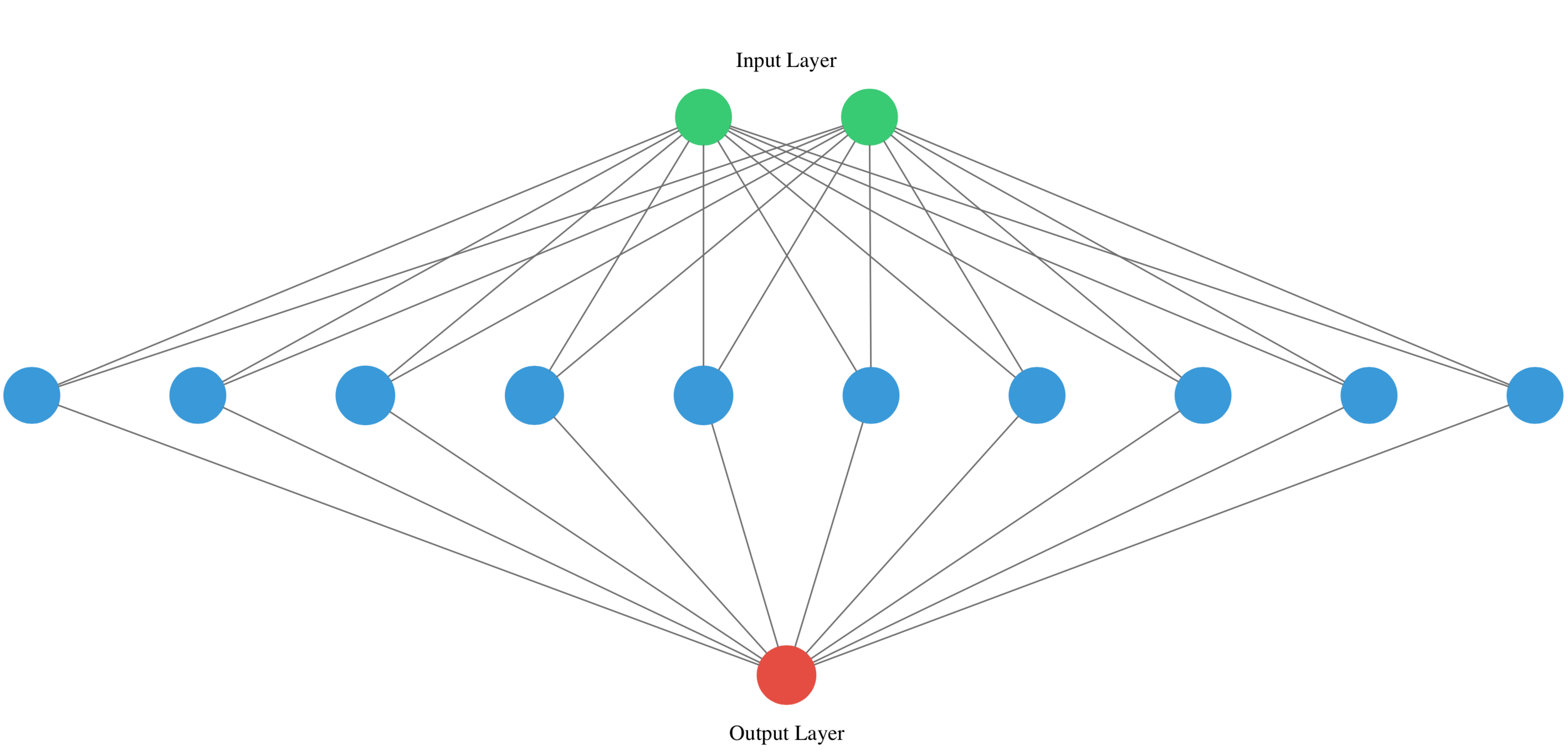
# Import the Sequential model and Dense layer
from keras.models import Sequential
from keras.layers import Dense

# Create a Sequential model
model = Sequential()

# Add an input layer and a hidden layer with 10 neurons
model.add(Dense(10, input_shape=(2,), activation="relu"))

# Add a 1-neuron output layer
model.add(Dense(1))

# Summarise your model
model.summary()
Model: "sequential_1"
_________________________________________________________________
Layer (type)                 Output Shape              Param #
=================================================================
dense_1 (Dense)              (None, 10)                30
_________________________________________________________________
dense_2 (Dense)              (None, 1)                 11
=================================================================
Total params: 41
Trainable params: 41
Non-trainable params: 0
_________________________________________________________________
You’ve just build your first neural network with Keras, well done!
1.2.2 Counting parameters
You’ve just created a neural network. Create a new one now and take some time to think about the weights of each layer. The Keras Dense layer and the Sequential model are already loaded for you to use.
This is the network you will be creating: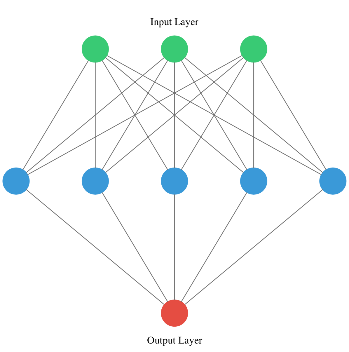
# Instantiate a new Sequential model
model = Sequential()

# Add a Dense layer with five neurons and three inputs
model.add(Dense(5, input_shape=(3,), activation="relu"))

# Add a final Dense layer with one neuron and no activation
model.add(Dense(1))

# Summarize your model
model.summary()
Model: "sequential_1"
_________________________________________________________________
Layer (type)                 Output Shape              Param #
=================================================================
dense_1 (Dense)              (None, 5)                 20
_________________________________________________________________
dense_2 (Dense)              (None, 1)                 6
=================================================================
Total params: 26
Trainable params: 26
Non-trainable params: 0
_________________________________________________________________
Given the model you just built, which answer is correct regarding the number of weights (parameters) in the hidden layer?
There are 20 parameters, 15 from the connection of our input layer to our hidden layer and 5 from the bias weight of each neuron in the hidden layer.
Great! You certainly know where those parameters come from!
1.2.3 Build as shown!
You will take on a final challenge before moving on to the next lesson. Build the network shown in the picture below. Prove your mastered Keras basics in no time!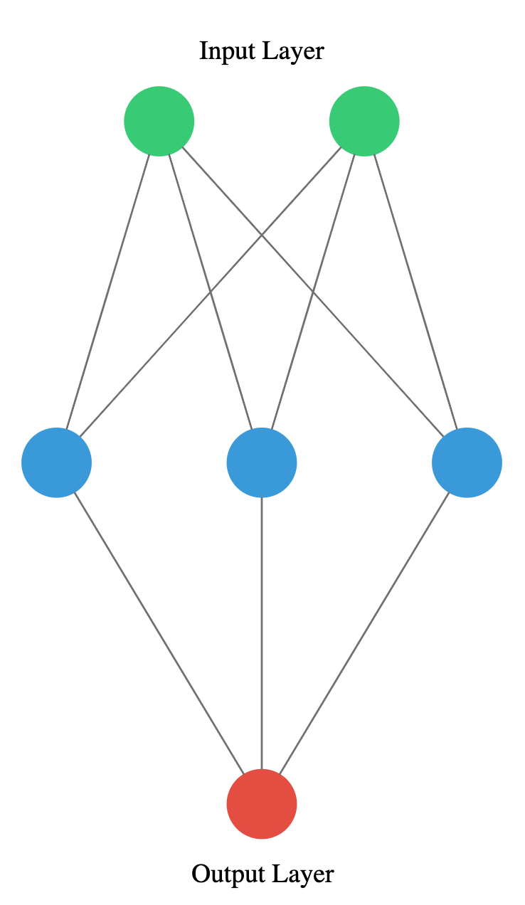
from keras.models import Sequential
from keras.layers import Dense

# Instantiate a Sequential model
model = Sequential()

# Build the input and hidden layer
model.add(Dense(3, input_shape=(2,)))

# Add the ouput layer
model.add(Dense(1))
Perfect! You’ve shown you can already translate a visual representation of a neural network into Keras code.
1.3 Surviving a meteor strike


1.3.1 Specifying a model
You will build a simple regression model to forecast the orbit of the meteor!
Your training data consist of measurements taken at time steps from -10 minutes before the impact region to +10 minutes after. Each time step can be viewed as an X coordinate in our graph, which has an associated position Y for the meteor at that time step.
Note that you can view this problem as approximating a quadratic function via the use of neural networks.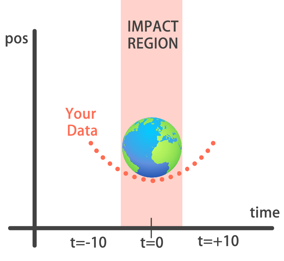
This data is stored in two numpy arrays: one called time_steps , containing the features, and another called y_positions, with the labels.
Feel free to look at these arrays in the console anytime, then build your model! Keras Sequential model and Dense layers are available for you to use.
# Instantiate a Sequential model
model = Sequential()

# Add a Dense layer with 50 neurons and an input of 1 neuron
model.add(Dense(50, input_shape=(1,), activation='relu'))

# Add two Dense layers with 50 neurons and relu activation
model.add(Dense(50,activation='relu'))
model.add(Dense(50,activation='relu'))

# End your model with a Dense layer and no activation
model.add(Dense(1))
You are closer to forecasting the meteor orbit! It’s important to note we aren’t using an activation function in our output layer since y_positions aren’t bounded and they can take any value. Your model is performing regression.
1.3.2 Training
You’re going to train your first model in this course, and for a good cause!
Remember that before training your Keras models you need to compile them. This can be done with the .compile() method. The .compile() method takes arguments such as the optimizer, used for weight updating, and the loss function, which is what we want to minimize. Training your model is as easy as calling the .fit() method, passing on the features, labels and number of epochs to train for.
The model you built in the previous exercise is loaded for you to use, along with the time_steps and y_positions data.
# Compile your model
model.compile(optimizer = 'adam', loss = 'mse')

print("Training started..., this can take a while:")

# Fit your model on your data for 30 epochs
model.fit(time_steps,y_positions, epochs = 30)

# Evaluate your model
print("Final lost value:",model.evaluate(time_steps, y_positions))
Training started..., this can take a while:
Epoch 1/30

  32/2000 [..............................] - ETA: 14s - loss: 2465.2439
 928/2000 [============>.................] - ETA: 0s - loss: 1820.2874
1856/2000 [==========================>...] - ETA: 0s - loss: 1439.9186
2000/2000 [==============================] - 0s 177us/step - loss: 1369.6929
...

Epoch 30/30

  32/2000 [..............................] - ETA: 0s - loss: 0.1844
 896/2000 [============>.................] - ETA: 0s - loss: 0.2483
1696/2000 [========================>.....] - ETA: 0s - loss: 0.2292
2000/2000 [==============================] - 0s 62us/step - loss: 0.2246
  32/2000 [..............................] - ETA: 1s
1536/2000 [======================>.......] - ETA: 0s
2000/2000 [==============================] - 0s 44us/step
Final lost value: 0.14062700100243092
Amazing! You can check the console to see how the loss function decreased as epochs went by. Your model is now ready to make predictions.
1.3.3 Predicting the orbit!
You’ve already trained a model that approximates the orbit of the meteor approaching earth and it’s loaded for you to use.
Since you trained your model for values between -10 and 10 minutes, your model hasn’t yet seen any other values for different time steps. You will visualize how your model behaves on unseen data.
To see the source code of plot_orbit, type the following print(inspect.getsource(plot_orbit)) in the console.
Remember np.arange(x,y) produces a range of values from x to y-1.
Hurry up, you’re running out of time!
# Predict the twenty minutes orbit
twenty_min_orbit = model.predict(np.arange(-10, 11))

# Plot the twenty minute orbit
plot_orbit(twenty_min_orbit)
# Predict the twenty minutes orbit
eighty_min_orbit = model.predict(np.arange(-40, 41))

# Plot the twenty minute orbit
plot_orbit(eighty_min_orbit)

Your model fits perfectly to the scientists trajectory for time values between -10 to +10, the region where the meteor crosses the impact region, so we won’t be hit! However, it starts to diverge when predicting for further values we haven’t trained for. This shows neural networks learn according to the data they are fed with. Data quality and diversity are very important. You’ve barely scratched the surface of what neural networks can do. Are you prepared for the next chapter?
